[4주차] 딥 러닝 구조 (데이터 정규화)

 딥 러닝의 오버피팅을 제어하는 데이터 정규화

딥 러닝(Deep Learning) 활용 시 거의 모든 함수가 표현 가능한 유연성이 있다. 하지만, 치명적인 단점으로 거론되는 오버피팅(Overfitting) 문제를 해결하기 위한, 다양한 정규화 기법들을 소개하도록 한다.

 

 ① Regularization (정규化, 정칙化)

Neural Net 계열은 오버피팅의 문제가 정말 중요하다. 따라서, 매 Layer 를 거듭함으로써 요동치는(Vanishing, Exploding) parameter 제약을 걸어 오버피팅을 방지하도록 한다. 특히, 이미지의 경우 학습 데이터 형태가 한정적일 수 있는데 약간의 변화를 줌으로써 비 지도학습 기반의 데이터 증강(Data Augmentation) 모형을 같이 소개하도록 한다.

 

• Regularization
- 추정하고자 하는 weight 에 제약을 가한다.
- DNN ≃ Universal function approximator.
   -. 학습 데이터 셋에 대하여 표현력이 아주 좋아짐 ⇒ overfitting 문제

- training dataset {(${𝑥}^{𝑖}$, ${𝑦}_{𝑖}$)} ${}_{}{}^{}_{𝑖=1}^{𝑛}$ 에 대해 Loss(data loss) $\sum _{𝑖=1}^{𝑛}{𝐿}_{𝑖}$ 를 최소화하는 parameter 𝑤 는 unique 하지 않다.
- unique 한 최적해를 얻기 위해 parameter 에 제약을 가하는데 이것을 regularizatin 이라고 한다. 이에 대한 손실을 regularization loss 라고 한다.
$$\begin{array}{r}\Rightarrow TotallossL=\underset{dataloss}{\underbrace{\frac{1}{N}\sum {𝐿}_{𝑖}}}+\underset{regularizationloss}{\underbrace{𝜆\Omega (𝜽)}}\\ \text{𝜆 is regularization strength}\end{array}$$
• Regularization 효과
  ⅰ) unique 한 solution 을 얻는다.
  ⅱ) smoothness of the prediction function
  ⇒ similar inputs produce similar outputs (부드러운 입/출력)
  ⅲ) overfitting 을 방지하여 generalization performance 를 높인다.
  ⇒ 즉, test error 를 줄인다. (for unknown data)
※ 정규화는 선택 사항이 아니고 거의 필수로 고려하는 사항이다.
EX)
  1) L2 Regularization ⋯ $\Omega (𝑤)={{\Vert 𝑤\Vert }_2}^2$
  ⇒ avoid peek weight vectors and prefering diffuse weight vectors
  특별한 벡터 값만 크게 나오는 문제를 피할 수 있다.
  L-2 Regression : Ridge Regression
  $$\begin{array}{r}L=\frac{1}{2}\sum {({𝑦}_{𝑖}-𝑓({𝑥}^{𝑖}))}^2+\frac{1}{2}𝜆{{\Vert 𝑤\Vert }_2}^2\end{array}$$
  2) L1 Regularization ⋯ $\Omega (𝑤)={\Vert 𝑤\Vert }_1$
  ⇒ sparse weight vectors (zero 성분이 많다)
  $${𝑤}^{\ast }=\left[\begin{array}{c}1\\ 0\\ ⋮\\ 0\\ 1\\ ⋮\\ 0\end{array}\right]\text{feature selection 에 사용 (extract non-zero)}$$
  3) Max norm ⋯ ${\Vert 𝑤\Vert }_2\le {𝐶}_{(Max)}$
※ 딥 러닝은 정규화를 하지 않으면 거의 오버 피팅이 일어나므로 꼭 주의해야 한다.

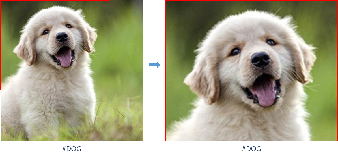
• Data Augmentation
  • Image Classification (컴퓨터 비전에서 이미지 분류는 상당히 어려움)
  - view point, lighting, occlusion, back-ground, scale 등에 따라 같은 클래스에서도 다양한 이미지가 존재한다.
  - 이러한 모든 형태의 training data 를 준비하는데 많은 시간과 비용이 들어감
  ⇒ 가지고 있는 training data 를 이용해서 training dataset size 증가시키는 것
[Define] Data augmentation refers to any method that artificially inflate the original training data with a label preserving transformation 𝜙 :
    𝜙 : 𝒮 → ℐ
𝒮: the original training dataset
ℐ: the augmented set of 𝒮
⇒ The final augmented training dataset 𝒮'
    𝒮' = 𝒮 ∪ ℐ
with labels preserved by 𝜙:
    (𝑥, 𝑦) ∈ 𝒮 $\stackrel{𝜙}{\to }$ (𝜙(𝑥), 𝑦) ∈ ℐ
※ 즉, 9 를 뒤집어서 변형된 6 이 레이블이 되는 경우는 피해야 한다.
1) Geometric transformations (기하학적 변형)
 -. x'=Ax+b : affine transformation (아핀 변환)
    b를 안 쓰기 위해서, $\left[\begin{array}{c}{x}^{\prime }\\ 1\end{array}\right]=\left[\begin{array}{cc}A& b\\ 0& 1\end{array}\right]\left[\begin{array}{c}x\\ 1\end{array}\right]$

  • reflection (flipping) - 반사 (뒤집기)
  • rotation - 회전
  • scaling - 크기를 줄이는 것
  • translation (when, b≠0) - 이동
  • shearing (skewing) - 찌그러 트리는 것

2) Color space transformation (photometric transformation)
 -. RGB channel 을 분리, gray-scale 만들기
 -. Lighting 조정 : pixel 값 조정 (0~255; black~white)
 -. Color histogram 조정 : 여러 프로그램에서 지원 됨

3) 기타
 -. cropping (자르기) - label 고정 후 학습

fixed label and cropping for augmentation

 -. noise injection (노이즈 삽입)
    { 𝑥' = 𝑥+θ, θ~𝑁(0, Σ) } ⋯ white noise
 -. kernel filter (대비) - 엣지를 선명하거나 흐리게 함
    { contrast, sharpening, blurring }
 -. mixing image (모자이크)
    { random image cropping + patching }
 -. random erasing (지우기)

* Unsupervised learning 이용한 training data 생성 (DNN 모형)
 • Restricted Boltzmann Machine (RBM)
 • Deep Belief Network (DBN)
 • Autoencoders
 • Generative Adversarial Network (GAN)

 

 ② Batch-Normalization (배치 정규화; ioffe & szegedy, 2015)

정규화의 또 다른 기법 중 하나인, 배치 정규화로써 다른 점은 parameter 제약을 걸지 않고 Test Error 를 줄이는 데 의의가 있다. 최종 목적인 오버피팅을 방지하기 위해서 입력 데이터 전처리(Dataset Shift)를 통해 광역 데이터를 손 봄으로써 딥러닝의 약점을 극복해보도록 한다.

 

[Define] Dataset Shift
distribution of training dataset {(${𝑥}^{𝑖}$, ${𝑦}_{𝑖}$)} ${}_{}{}^{}_{𝑖=1}^{𝑛}$ ≠ distribution of test dataset (𝑥,𝑦)
* Dataset Shift 가 일어나면 Supervised learning 의 기본 가정이 깨진다.
$$\begin{array}{r}{({𝑥}^{𝑖},{𝑦}_{𝑖})}_{training}:𝑖=1,\cdots ,𝑛;\text{ 𝑖.𝑖.𝑑 copies of }(𝑥,𝑦)\in P_{test}\end{array}$$
⇒ 지도학습의 기본 가정이 깨지지만, 실제로도 시간에 따라 데이터 분포는 바뀌기 마련이다. (흔한 문제)
* 다른 용어로는 concept drift, concept shift, covariate shift, non-stationality
* Types of dataset shift
 ① shift in independent variables X → {covariate shift}¹ (독립 변수 분포 변화)
 ② shift in the target variables Y → {prior distribution shift}² (종속 변수 분포 변화)
 ③ shift in the relationship between X and Y → {concept shift} (예측 함수의 변화)
* Recall Bayse formula
$$\begin{array}{r}P(𝑦,𝑥)=\frac{𝑓(𝑥|𝑦)𝜋(𝑦)²}{𝑓(𝑥)¹}\end{array}$$
[Define] Internal Covariate Shift
covariate shift in the given training dataset {(${𝑥}^{𝑖}$, ${𝑦}_{𝑖}$)} ${}_{}{}^{}_{𝑖=1}^{𝑛}$
⇒ DNN 에서 original 입력 {(${𝑥}^{𝑖}$, ${𝑦}_{𝑖}$)} 에 대하여 각 Layer 에 입력되는 data 의 분포가 달라지는 경우 

각 레이어 별 분포가 달라지면 깊어질수록 아주 안좋은 현상이 일어난다.

 * Internal Covariate Shift Cause
  ① delay training (학습이 오래 걸림)
  ② lower learning rate (학습 속도가 현저히 떨어짐)
  ③ careful about initialization (파라미터 초기화 결과가 민감해짐)
 * How to avoid internal covariate shift ?
  → Normalization : the process of scaling down the data to some reasonable limit to standize the range of ${𝑥}_{𝑗}$
 $$\begin{array}{r}{\widehat{𝑥}}_{𝑗}=\frac{{𝑥}_{𝑗}-E{𝑥}_{𝑗}}{\sqrt{Var{𝑥}_{𝑗}}}⇝𝑁(0,1)\end{array}$$
  - 각 레이어에 입력 될 때마다 Normalization 을 feature 별로 해 준다.
 * The effect of normalization : reduce the effect of exploding and vanishing gradient
※ 최근 논문에 의하면 loss function 의 gradient 𝛻𝑤𝐿 를 Lipschitz continuous 하게 한다.
⇒ normalization 이 internal covariate shift 를 줄이는 것은 아니다.
※ 여기서 Batch 의미는 mini-Batch 를 의미한다. 즉, 𝑛 개의 examples (sample points) 에서 subset (mini-batch) 을 취하여 normalize 한다.

• Batch Normalization Algorithm
-. Training Dataset : {${𝑥}^{𝑖}$} ${}_{}{}^{}_{𝑖=1}^{𝑛}$, ${𝑥}^{𝑖}$∈$R^D$
Batch Normalization of feature 𝑗 ∈ {1,⋯,𝒟}
Input : mini-batch 𝒮 of size 𝑚
    |𝒮| = 𝑚
Output : ${𝑦}_{𝑗}^{𝑖}=𝐵{𝑁}_{{\gamma }_{𝑗},{\beta }_{𝑗}}$ $({𝑥}_{𝑗}^{𝑖})$, 𝑖∈𝒮
    $${\mu }_{𝑗}=\frac{1}{𝑚}\sum _{𝑖\in S}{𝑥}_{𝑗}^{𝑖}\text{ ⋯ mini-batch mean}$$
    $${\sigma }_{𝑗}^2=\frac{1}{𝑚}\sum _{𝑖\in S}{({𝑥}_{𝑗}^{𝑖}-{\mu }_{𝑗})}^2\text{ ⋯ mini-batch var}$$
    $${\widehat{𝑥}}_{𝑗}^{𝑖}=\frac{({𝑥}_{𝑗}^{𝑖}-{\mu }_{𝑗})}{\sqrt{{\sigma }_{𝑗}^2}},𝑖\in S\text{ ⋯ normalization}$$
    $$\begin{array}{rl}{𝑦}_{𝑗}^{𝑖}& ={\gamma }_{𝑗}{\widehat{𝑥}}_{𝑗}^{𝑖}+{\beta }_{𝑗}\\ & =\frac{{\gamma }_{𝑗}}{\sqrt{{\sigma }_{𝑗}^2}}{𝑥}_{𝑗}^{𝑖}+({\beta }_{𝑗}-\frac{{\gamma }_{𝑗}{\mu }_{𝑗}}{\sqrt{{\sigma }_{𝑗}^2}})\\ & \triangleq 𝐵{𝑁}_{{\gamma }_{𝑗},{\beta }_{𝑗}}({𝑥}_{𝑗}^{𝑖})\text{ ⋯ scale and shift}\end{array}$$
* ${\gamma }_{𝑗},{\beta }_{𝑗}$ 는 network parameter 와 함께 training 한다.
* activation (e.g., ReLU) 에 들어가기 전에 각 레이어 입력에 대하여 실행.
* Test data 에 대해서는 Training data 의 평균과 분산을 이용한다.
* DNN, 특히 CNN 에서는 필수적으로 적용되며 𝐵𝑁 𝐿𝑎𝑦𝑒𝑟 라고 한다.

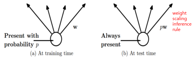
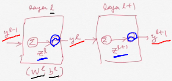
• Dropout : Stochastic Regularization (Hinton, 2012)
-. Basic idea : Dropping out units (hidden and visible) in a neural network

dropout

 * 어떤 unit 을 dropout 하면 그 unit 에 들어오는 연결과 나가는 연결을 모두 제거한다.

(a) unit 이 확률 p로 제어됨 (node 제거), (b) node 그대로 두고 weight scaling

 [Model description]
 {1,⋯,𝐿} : the index of hidden layer
 ${𝑧}^{\ell }$ : input vector into layer ℓ
 ${𝑦}^{\ell }$ : output vector from layer ℓ
     { ${𝑦}^0$ = 𝑥 : original input }
 ${𝑤}^{\ell }$ : weight matrix of layer ℓ
 ${𝑏}^{\ell }$ : bias vector of layer ℓ

input vector z into activation function of layer ℓ

1) Standard neural network For any hidden layer 𝑖
 ${𝑧}_{𝑖}^{\ell +1}$ = ${({𝑤}_{𝑖}^{\ell +1})}^{𝑇}{𝑦}^{\ell }+{𝑏}_{𝑖}^{\ell +1}$
 ${𝑦}_{𝑖}^{\ell +1}$ = $𝜑({𝑧}_{𝑖}^{\ell +1})$

2) Dropout
 ${𝑟}_{𝑖}^{\ell }$~𝐵𝑒𝑟𝑛(𝑃)
 ${\widetilde{𝑦}}^{\ell }$ = ${𝑟}^{\ell }\bullet {𝑦}^{\ell }$
    𝑋~𝐵𝑒𝑟𝑛(𝑃) ⋯ 베르누이 분포 정의
    𝑝𝑑𝑓 of 𝑋 : 𝑓(𝑥) = 𝑃${}^{𝑥}$(1-𝑃)${}^{1-𝑥}$
    $𝑟\bullet 𝑦$ ⋯ dot product 정의 : 컴포넌트들의 곱
 ${𝑧}_{𝑖}^{\ell +1}$ = ${({𝑤}_{𝑖}^{\ell +1})}^{𝑇}{\widetilde{𝑦}}^{\ell }+{𝑏}_{𝑖}^{\ell +1}$
 ${𝑦}_{𝑖}^{\ell +1}$ = $𝜑({𝑧}_{𝑖}^{\ell +1})$
 (𝑖 번째 component 를 zero 로 하는 것은 layer (ℓ-1) 의 𝑖 번째 unit 을 제거하는 것과 같다)

𝑟 곱에 따라 랜덤하게 컴포넌트가 hidden/visible 된다.

* At test time, the weights are scaled as ${𝑤}_{test}^{\ell }=𝑃{𝑤}^{\ell }$

 • Dropout Training
 {ℎ₁,⋯,ℎ𝑚} : 𝑛 layer
 Θ = {𝜽₁,⋯,𝜽𝑛} : 𝜽𝑖 the matrix of 𝑖-th layer parameter
 𝜎 = {𝜎₁,⋯,𝜎𝑛} : 𝜎𝑖 configuration of layer 𝑖
     ex) 𝜎𝑖 : 0-1 vector denoting dropping of units in the 𝑖-layer

Representation units in the hidden layer 𝑖

 -. Each layer is a function defined by ℎ𝑖(𝑧) = 𝑎(𝜽𝑖${}^{𝑇}$𝑧) ⋯ 𝑎(·) : activation function
 -. The composition of layer 𝑓${}_{\Theta }$ = ℎ𝑛 º ℎ𝑛-₁ º ⋯ º ℎ₁ : 𝒳→𝒴

유닛이 죽고 살아나는 것을 각 컨피그레이션 별 시그마로 나타낼 수 있다.

 ⇒ The thinned neural network (sub-network) parameterized by Θ with configuration 0-1 variable 𝜎 = {𝜎₁,⋯,𝜎𝑛} : 𝑓${}_{\Theta ,𝜎}$
     $$\{\begin{array}{ll}& \text{ℎ𝑖(𝑧) = 𝜎𝑖 • 𝑎(𝜽𝑖}{}^{𝑇}\text{𝑧)}\\ & \text{𝑓}{}_{\Theta ,𝜎}\text{ = ℎ𝑛 º ℎ𝑛-₁ º ⋯ º ℎ₁}\end{array}$$
 -. The goal of dropout training (최적의 파라미터를 찾는다)
     Θ* = $\underset{\Theta }{\arg \min }$ 𝑅(Θ)
 $$\begin{array}{rl}𝑅(\Theta )& ={𝔼}_{𝑥,𝑦,𝜎}𝐿(Y,{𝑓}_{\Theta ,𝜎}(X))\\ & \text{𝜎 ~ 𝐵𝑒𝑟𝑛(𝑃)}\\ & \text{ℐ : training dataset}={}_{}{}^{}\{({𝑥}^{𝑖},{𝑦}_{𝑖})\}_{𝑖=1}^{𝑛}\end{array}$$
⇒ Empirical Risk
 $${𝑅}_{𝑛}(\Theta )=\frac{1}{𝑛}\underset{𝑖=1}{\sum ^{𝑛}}{𝔼}_{𝜎}𝐿({𝑦}_{𝑖},{𝑓}_{\Theta ,𝜎}({𝑥}^{𝑖}))$$

Algorithm : Dropout Training
1. Input : Training dataset ℐ = {(${𝑥}^{𝑖}$, ${𝑦}_{𝑖}$)} ${}_{}{}^{}_{𝑖=1}^{𝑛}$
2. 𝑡 = 0
3. Initialize network parameter Θ${}^0$
4. Repeat
5. Sample {(${𝑥}^{{𝜋}_1}$, ${𝑦}_{{𝜋}_1}$),⋯,(${𝑥}^{{𝜋}_{𝑚}}$, ${𝑦}_{{𝜋}_{𝑚}}$)}
    ⊂ ℐ : mini-batch of size 𝑚
6. Sample dropout variable ${𝜎}^1,\cdots ,{𝜎}^{𝑚}$
    ${𝜎}^{𝑗}$ : 𝑗-th sample point 의 dropout
7. Update learning rate ${\eta }_{𝑡}$
8. Update network parameter
    ${\Theta }^{𝑡+1}={\Theta }^{𝑡}-\frac{{\eta }_{𝑡}}{𝑚}\sum _{𝑗=1}^{𝑚}\frac{\partial }{\partial \Theta }𝐿({𝑦}_{{𝜋}_{𝑗}},{𝑓}_{{\Theta }^{\ast },{𝜎}^{𝑗}}({𝑥}^{{𝜋}_{𝑗}}))$
9. 𝑡 = 𝑡+1
10. Until : Stopping criterion is met.
11. Output : ${\Theta }^{\ast }={\Theta }^{𝑡}$
* Dropout 은 각 sample point 마다 독립적으로 일어난다.