딥 러닝(Deep Learning) 기초 개념인 MLP(Multi Layer Perceptron) 내용에 대해 학습하였다. 이제부터는 Hidden Layer 개수를 추가(L ≥ 2)하여 비선형 문제를 포함한 복잡한 함수를 표현할 수 있게 되었다. 이에 따라, 발생될 수 있는 오버 피팅을 정규화로 제어하고, 딥 러닝을 활용한 다중 클래스 분류(Multiclass Classification) 2 가지를 보도록 한다.
① Structure of MLP, (L=2)
본격적으로 머신 러닝의 한 부분인 딥 러닝 구조에 대해서 학습하고, 최적 파라미터에 접근하는 방법에 대해 알아보도록 한다.
• Structure of Layers (input → hidden 1 → hidden 2 → output) \(𝑥∈𝑅^D\) → \(𝑓∈𝑅^K\) → [M/L model] → compute loss L \[ 𝑤= \begin{bmatrix} 𝜔^1, ⋯, 𝜔^J \end{bmatrix}\, \, \, D×J \] \[ 𝑢= \begin{bmatrix} 𝜇^1, ⋯, 𝜇^𝑃 \end{bmatrix}\, \, \, J×P \] \[ 𝑣= \begin{bmatrix} 𝑣^1, ⋯, 𝑣^𝐾 \end{bmatrix}\, \, \, P×K \] * output layer 에서는 activation 을 하지 않는다. 단순 합만 주로 계산한다. * MLP(DNN) contains multiple non-linear hidden layers ⇒ very expressive model that can be learn very complicated relationships between input and outputs ⇒ DNN is a universal function approximator ! ※ 모든 트레이닝 데이터를 fitting 할 수 있는 표현력이 좋지만, overfitting 을 조심해야 한다 !
② Multi-class classification using DNN
가령, 신경망 구조를 통해 이미지를 보고 동물을 구분해야 한다고 하자. 여태까지의 이진 분류(개 이거나, 개가 아니거나)가 아닌, 다중 클래스 분류(개/고양이/닭 등)를 위해 해당 결과(class)에 대한 점수(score) 개념이 필요하다. 따라서, 해당 이미지가 주어진 class에 얼마나 적합한지 나타내는 점수에 대해 학습하고, 이 점수의 오차를 설명해주는 Loss Function 2가지(SVM vs. Softmax) 경우를 살펴보고 정확도를 높이기 위한 파라미터를 찾아보도록 한다.
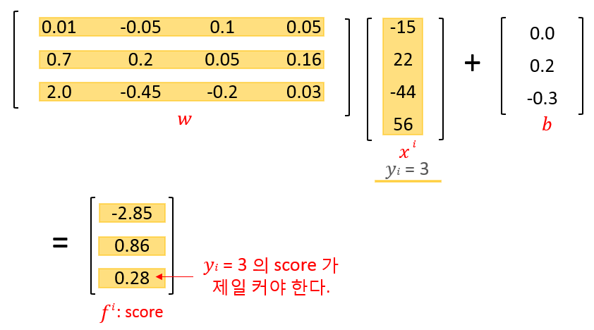
The score for the 𝑘-th class given \(𝑥^𝑖\) ⋯ sample point \(𝑥^𝑖\)가 주어졌을 때, class 𝑘 에 들어가는 점수 \[ {𝑓(𝑥^𝑖; 𝑤,𝑏)}_𝑘 ≜ 𝑓_𝑘^𝑖 = {(𝜔^𝑘)}^𝑇𝑥^𝑖 +𝑏_𝑘 \]
※ Interpretation of score - The correct class has a score that is higher than the scores of incorect class -. class 𝑘 점수가 다른 class 점수보다 높도록 한다. ⋯ class 𝑘 has a highest score - The training data is used to learn the parameters (𝑤,𝑏) for that purpose -. 즉, 올바른 클래스의 점수가 커지도록 파라미터를 최적화시켜야 한다. ⇒ \({(𝑥^𝑖, 𝑦_𝑖)}\)에 대하여 \(𝑥^𝑖\)의 score 가 \(𝑦_𝑖\) class 에서 최대가 되도록 (𝑤,𝑏) 를 정해준다.
EX. mapping on image to class score [CS231n] ⇒ score 계산 결과를 보면, \(𝑥^𝑖\) 의 class 가 class 2 인것 처럼 보인다. 그러나, 실제 class 는 \(𝑦_𝑖\)=1 이므로 class 1 이다. 따라서, 현재 weight 𝑤 와 bias 𝑏 는 적절치 않다. ⇒ (𝑤,𝑏) 를 update 해서 class 1 의 score 가 최대가 되도록 해야한다. ※ loss function 을 잘 정의해서 loss 를 최소화 함으로써 이러한 목적이 달성되도록 함 - Define loss function to measure our unhappiness with outcomes such as this. - We consider two loss function. ① SVM loss ② Softmax loss
① Multiclass SVM loss (hinge loss 또는 margin error) hinge loss - The multi-class SVM loss for the 𝑖-th example: \[ \eqalign{ 𝐿_𝑖 &= \sum\limits_{𝑘 ≠ 𝑦_𝑖} max{(0, 𝑓_𝑘^𝑖 - 𝑓_{𝑦_𝑖}^𝑖 + △)} \\ &= \sum\limits_{𝑘 ≠ 𝑦_𝑖} {(𝑓_𝑘^𝑖 - 𝑓_{𝑦_𝑖}^𝑖 + △)}_+ } \] - The multi-class SVM wants the score of the correct class to be higher than all other classes by at least a margin of data * hinge loss [margin error] 구하는 법 - 𝑇𝑖𝑝 1) Must be☆ > △ 2) 음수化 + margin(△-☆ +γ) 3) ReLU化 : hinge loss = (△-☆ -γ)\({}_+\)
② Softmax classifier (cross entropy loss function) ≒ Multiclass logistic regression:𝒴 = {1, 2, ⋯, 𝐾} - Basic idea: feature vector 𝑥 가 주어졌을 때, class 의 posterior 분포 𝑃(𝑌=𝑗|𝑋=𝑥) ≜ 𝑃(𝑗|𝑥) 를 추정한다. (추정치 𝑝̂(𝑗|𝑥), 𝑗=1,⋯,𝐾) ⇒ Final classifier: \[ 𝑔(𝑥) = arg\, \operatorname*{max}\limits_{𝑗 ∈ 𝑦}\, {\color{Red}𝑝̂(𝑗|𝑥)} \] - Define 𝑝̂(𝑗|𝑥):estimated class probability given 𝑋=𝑥 \[ log\frac{𝑝̂(𝑗|𝑥)}{𝑍} = {(𝜔^𝑗)}^𝑇𝑥 +𝑏_𝑗 ≜ {\color{Red}𝑓_𝑗 \, \, ⋯ \mbox{score}} \] ※ when 𝑍 : normalization constant ⇒ 𝑝̂(𝑗|𝑥) = \(𝑍e^{𝑓_𝑗}\) ⇒ \(\sum\limits_{𝑗=1}^{𝐾} 𝑝̂(𝑗|𝑥)\) = \(𝑍 \sum\limits_{𝑗=1}^{𝐾} e^{𝑓_𝑗}\) = 1 ⇒ 𝑝̂(𝑗|𝑥) = \(\frac{e^{𝑓_𝑗}}{\sum\limits_{𝑘=1}^{𝐾} e^{𝑓_𝑘}}\) ≜ \({\color{Red}softmax(𝑓)_𝑗}\) ≜ \({\color{Red}𝜎(𝑓)_𝑗}\) , 𝑗=1,⋯,𝐾 ※ estimation 은 위와 같고, 총 합은 1 과 같다. (※ sigmoid 첨자와 구분: \(𝜎(𝑓_𝑗)\) = \(\frac{1}{1+e^{-𝑓_𝑗}})\)
- True class probability given (𝑥, 𝑦) ⋯ sample ※ 다음으로, True 분포는 (True 는 모르기 때문에 샘플을 뽑아 실측치로 보겠다.) \[ 𝑃(𝑗|𝑥) = \begin{cases} 1, & 𝑗=𝑦 \\ 0, & \mbox{otherwise} \end{cases} {\color{Red} \cdots \mbox{ground truth (실측치)}} \] - Density estimation using cross entropy ※ estimation 추정치를 true 실측치에 가깝게 만들어주면 된다. \[ \eqalign{ H(𝑃, 𝑝̂) &≜ \sum\limits_{𝑗=1}^{𝐾} 𝑃(𝑗|𝑥) \, log \, \frac{1}{𝑝̂(𝑗|𝑥)} \\ &= -log \, 𝑝̂(𝑦|𝑥) } \] ⇒ CE loss for the sample point (𝑥, 𝑦) \[ \eqalign{ 𝐿 &= -log \, \frac{e^{𝑓_𝑦}}{\sum\limits_{𝑘=1}^{𝐾} e^{𝑓_𝑘}} \\ &= -𝑓_𝑦 + log \, \sum\limits_{𝑘=1}^{𝐾} e^{𝑓_𝑘} } \]
2) Training dataset {(\(𝑥^𝑖\), \(𝑦_𝑖\))} \(\sideset{_{}^{}}{_{𝑖=1}^𝑛}{}\) 에 대한 loss -. CE loss for an example (\(𝑥^𝑖\), \(𝑦_𝑖\)) \[ \eqalign{ 𝑝̂(𝑦_𝑖|𝑥^𝑖) &= \frac{e^{𝑓_{𝑦_𝑖}^𝑖}}{\sum\limits_{𝑘=1}^{𝐾} e^{𝑓_𝑘^𝑖}} \\ &where, \, 𝑓_𝑘^𝑖 = {(𝜔^𝑘)}^𝑇𝑥^𝑖 +𝑏_𝑘 \, {\color{Red}: 입력이 𝑥^𝑖 일때 class \, 𝑘 의 score} } \] \[ \eqalign{ ⇒ 𝐿_𝑖 &= -log \, \frac{e^{𝑓_{𝑦_𝑖}^𝑖}}{\sum\limits_{𝑘=1}^{𝐾} e^{𝑓_𝑘^𝑖}} \\ &= -𝑓_{𝑦_𝑖}^𝑖 + log \, \sum\limits_{𝑘=1}^{𝐾} e^{𝑓_𝑘^𝑖} } \] Total loss\(𝐿 = \frac{1}{𝑛} \, \sum\limits_{𝑖=1}^{𝑛} \, 𝐿_𝑖 \)
Ex: 𝑖 번째 input 에 대한 score vector 𝒴={1, 2, 3, 4} ; 4 classes 만약, \(𝑥^𝑖\) 가 class 3 이면 loss = -log 0.0790 = 2.5383 class 2 이면 loss = -log 0.7876 = 0.2388 (바람직한 결과) * Total loss 가 최소가 되도록 각 class 의 weight \(𝑤^𝑘\) 와 bias \(𝑏_𝑘\) 를 계산. 만약, \(𝑥^𝑖\) 의 class 가 1 이고 \(𝑝̂(𝑗|𝑥^𝑖)\) 가 \(\begin{bmatrix} 1 \\ 0 \\ 0 \\ 0 \end{bmatrix}\) 형태이면, loss = zero 가 된다. 즉, 이 경우 추정치 \(𝑝̂(𝑗|𝑥^𝑖)\) 와 실측치(true 분포) \(𝑃(𝑗|𝑥)\) 가 일치한다.